Friedman test
Friedman test
The Friedman test tests the Nullhypothesis of identical populations for dependent data. It is an equivalent to the one factorial variance analysis with repeated measurement without making any assumptions on the distributions of the populations. It uses only the rank information of the data.
Requirements:
Data must be ordinal (rank-order) scaled. Distribution is free.
Hypothesis:
H0: The treatments have identical effects
H1: At least one treatment is different from at least one other treatment
Idea:
The data of k subjects and p treatments are first displayed in a two dimensional table. Then the data of each person are brought into one rank order (treatment ranks). This procedure ensures that the dependency of the data is taken into account. Next for each treatment the sum of ranks Ti is computed. Whereas the total sum of ranks is:
with
k = number of subjects
p = number of treatments
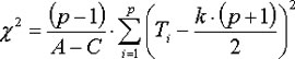
For sufficiently large sample sizes (k>10 and p>4) the following value is approximately Chi-Square distributed with p-1 degrees of freedom:
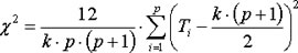
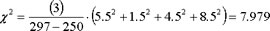
if there are tied ranks Chi-Square is computed the following way:

wheras
Conover recommends the following F statistic, which has a more accurate approximation:
with
 degrees of freedom
Post-hoc analysis
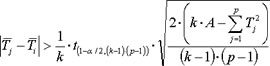
If the H0 is rejected it is often desirable to know which treatments are different from each other. Treatments i and j are different if the difference between the two mean ranks meets the following requirment:
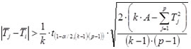
 = critical t-value with (k-1)(p-1) degrees of freedom
Example of a Friedman test
In a poll 10 subjects rated 4 different paintings on a scale from 0 (don’t like it at all) to 5 (like it very much). The following table shows the data and ranks for all tubjects and paintings:
| Paintings | ||||||||
| 1 |
Rank |
2 |
Rank |
3 |
Rank |
4 |
Rank |
|
| 1 |
0 |
1 |
5 |
4 |
1 |
2 |
4 |
3 |
| 2 |
3 |
2 |
4 |
3 |
2 |
1 |
5 |
4 |
| 3 |
1 |
1 |
4 |
3.5 |
3 |
2 |
4 |
3.5 |
| 4 |
4 |
4 |
2 |
1.5 |
2 |
1.5 |
3 |
3 |
| 5 |
2 |
1.5 |
2 |
1.5 |
4 |
4 |
3 |
3 |
| 6 |
0 |
1 |
3 |
2 |
5 |
3.5 |
5 |
3.5 |
| 7 |
3 |
2.5 |
1 |
1 |
3 |
2.5 |
4 |
4 |
| 8 |
5 |
3.5 |
3 |
2 |
1 |
1 |
5 |
3.5 |
| 9 |
1 |
1 |
5 |
4 |
2 |
2 |
4 |
3 |
| 10 |
2 |
2 |
4 |
4 |
0 |
1 |
3 |
3 |
| Ti |
19.5 |
26.5 |
20.5 |
33.5 |
||||
 |
1.95 |
2.65 |
2.05 |
3.35 |
||||
We then get for the total sum of ranks:
We have tied ranks so the Chi-square value is:
whereas
so the Chi-square value is:
The critical 5% Chi-square for 3 degrees of freedom is 7.81. The Chi-square test does reject H0. There must be at least one painting which is differentially rated compared to at least one other painting.
For Conovers’ F value we get:
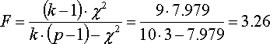
and the 5% critical F value with 3 and 27 degrees of freedom is 2.96. The F Test does reject H0. There must be at least one painting which is differentially rated compared to at least one other painting.
The critical Difference of the Mean Ranks is:
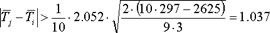
The following table shows the differences of the mean ranks:
| Painting 1 |
Painting 2 |
Painting 3 |
|
| Painting 2 |
0.7 |
- |
- |
| Painting 3 |
0.1 |
0.6 |
- |
| Painting 4 |
1.4 * |
0.7 |
1.3 * |
Post hoc paired comparisons reveal that painting four is rated differentially compared to paintings 1 and 3.
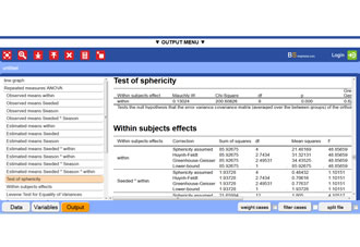
BrightStat output of Friedman test example
This is a fictitious example.
Wiki link Friedman test
References
Bortz, J. (2005). Statistik für Human- und Sozialwissenschaftler (6th Edition). Heidelberg: Springer Medizin Verlag.
Conover, W.J. (1999). Practical nonparametric Statistics.(3rd edition). Wiley.
Friedman, M. (1937). The use of ranks to avoid the assumption of normality implicit in the analysis of variance. Journal of the American Statistical Association (American Statistical Association), 32 (200), 675 – 701. doi:10.2307/2279372
Friedman, M. (1939). A correction: The use of ranks to avoid the assumption of normality implicit in the analysis of variance. Journal of the American Statistical Association (American Statistical Association), 34 (205), 109. doi:10.2307/2279169
Schaich, H.E. & Hamerle, A. (1984). Verteilungsfreie statistische Prüfverfahren, Berlin.


 Donate IOTA