one-way analysis of variance (ANOVA)
One-way analysis of variance (ANOVA)
In general, the term ANOVA describes a method to detect the influence of independent variables on one or more dependent variables. The ANOVA was first developed by Sir Ronald A. Fisher (1890 – 1962). In the context of ANOVA the independent variable is also called predictor variable, controlled variable, manipulated variable, explanatory variable, experimental factor or input variable and the dependent variable is also called response variable, measured variable, explained variable, experimental variable, responding variable, outcome variable or output variable. A one-way ANOVA is the simplest form of an ANOVA where the influence of one independent variable on one dependent variable is quantified. A one-way ANOVA may be considered as an extension of a t-test when more than two group means are to be compared.
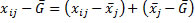
Sir Ronald A. Fisher’s main idea:
(1) 
Whereas:
 = Measurement of person i in group j
 = Mean of all measurements in group j
 = Grand mean of all measurements
Expressed in words this means that the difference of an individual measurement to the grand mean  can be explained as the difference of this individual’s measurement to the group mean
  plus the difference of the group mean to the grand mean
  . The first part describes the error which is not caused by the independent variable but by external and or subject variables. The second part stands for the influence of the independent variable on the dependent variable.
Example 1: 20 subjects, 4 treatments, no effect  , no
error
, no
error 
|
|
Treatment |
|||
|
|
1 |
2 |
3 |
4 |
|
|
4 |
4 |
4 |
4 |
|
|
4 |
4 |
4 |
4 |
|
|
4 |
4 |
4 |
4 |
|
|
4 |
4 |
4 |
4 |
|
|
4 |
4 |
4 |
4 |
|
Mean |
4 |
4 |
4 |
4 |
Example 2: 20 subjects, 4 treatments, effect (mean differences) but no errors
|
|
Treatment |
|||
|
|
1 |
2 |
3 |
4 |
|
|
2 |
3 |
7 |
4 |
|
|
2 |
3 |
7 |
4 |
|
|
2 |
3 |
7 |
4 |
|
|
2 |
3 |
7 |
4 |
|
|
2 |
3 |
7 |
4 |
|
Mean |
2 |
3 |
7 |
4 |
Example 3: 20 subjects, 4 treatments, possibly real data
|
|
Treatment |
|||
|
|
1 |
2 |
3 |
4 |
|
|
2 |
3 |
6 |
5 |
|
|
1 |
4 |
8 |
5 |
|
|
3 |
3 |
8 |
5 |
|
|
3 |
5 |
4 |
3 |
|
|
1 |
0 |
9 |
2 |
|
Mean |
2 |
3 |
7 |
4 |
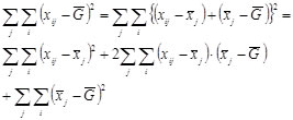
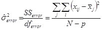
Because the sum of all differences for subjects 1 to n always add up to 0 we will square equation (1)
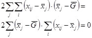
The middle term will always add up to 0:
So we get the sum of squares (SS):
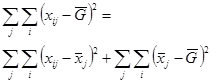
SSTotal = SSError + SSTreatment
Whereas nj is the number of measurements in group j.
Degrees of freedom
N-1 = (N-p) + (p-1)
Wheras N is the total number of subjects and p is the number of treatments.
Or in case that all groups are identical in size:
N-1 = n(p-1) + (p-1)
Wheras N is the total number of subjects, n is the number of subjects in each treatment group and p is the number of treatments.
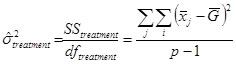
The sum of squares are then divided by the degrees of freedom to form the mean squares (MS)
MSError = SSError / dfError
MSTreatment = SSTreatment / dfTreatment
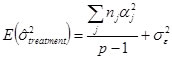
Population
For the population we consider the following model:
xij = μ + αj + εij a subject’s measurement
αj = μj - μ effect of treatment j
εij = xij - μj effect of confounding variables (error)
Assumptions
1) Errors εj are normally distributed in each treatment
2) Error variances are the same for each treatment (homogeneity of variances)
3) All pairs of errors within and between treatments are independent.
The above assumptions lead to the following population estimates:

The two variances (treatment and error) are compared using a Fisher’s F-test.
Hypotheses
H0: μ1 = μ2 = μ3 = ... μp (all αj = 0)
H1: not H0, there is at least one αj ≠ 0
Test

Degrees of freedom
numerator: p-1
denominator: N-p
If and only if group sizes are the same for all treatments the degrees of freedom of the denominator can also be written as p(n-1).
If the treatment effect is present, the variance in the numerator must be greater compared to the variance in the denominator. The F-value must then be greater than 1. Hence, the obtained F-value will always be compared to the right sided critical F-value of the corresponding F-distribution.
Presenting the results
|
Source |
SS |
df |
|
F |
p |
|
Treatment |
SSTreatment |
p-1 |
|
|
α |
|
Error |
SSError |
N-p |
|
|
|
|
Total |
SSTotal |
N-1 |
|
|
|
 (MS)
(MS)


Effect size
The effect size is a measure of strength between the treatment and the outcome. It is an estimate of the proportion of variance the two variables have in common.
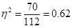
Eta-squared for the sample:

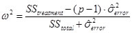
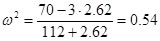
Omega squared for the population:
Difference between eta-squared  and partial eta-squared
  :
:
Partial eta-squared is often reported by statistical software like SPSS or others. In the context of a one-way ANOVA these two measures are identical. This will be obvious when you consider the following equation:
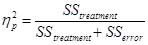
Wheras in an one-way ANOVA SStotal is defined as SStreatment+SSerror
In multifactorial ANOVAs there is more than one SStreatment
plus the SSs of all interactions. In those cases you must be careful not to
confound with .
A good summary of how eta-squared, partial-eta-squared and Cohen’s f are related is given here.
Post-hoc tests
When a significant result is obtained, the question arises which treatment(s) is(are) different from which other treatment(s). Or simply which αj is not zero.
Many different post-hoc tests have been developed for different purposes. When it is necessary to compare all pairs of means to get an idea which mean differences are significant, the Tukey HSD (Honest Significant Difference) test is the best choice, even if group sizes are not equal. If variance homogeneity is violated (this can be tested for example by the Levene-test), Games-Howell might be the best choice.
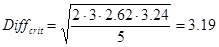
For the case of equal group sizes and equal error variances (variance homogeneity) the critical difference by Scheffé is a simple yet very conservative method to compare the group means:
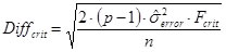
Whereas Fcrit = F(p-1; N-p; 1-α)
Example
Let’s assume that we have four different teaching methods we want to compare. We assign 5 out of 20 subjects randomly to each teaching method. After a semester we perform a test that we assume to measure what the subjects have learned during the semester. The test may give the following results (0 = very bad, 10 = excellent)
|
|
Teaching method |
|||
|
|
1 |
2 |
3 |
4 |
|
|
2 |
3 |
6 |
5 |
|
|
1 |
4 |
8 |
5 |
|
|
3 |
3 |
8 |
5 |
|
|
3 |
5 |
4 |
3 |
|
|
1 |
0 |
9 |
2 |
|
Mean |
2 |
3 |
7 |
4 |
Is there a teaching method that leads to significant better results compared to another one?
The ANOVA yields the following result table:
|
Source |
SS |
df |
|
F |
p |
|
Treatment |
70 |
3 |
23.33 |
8.89 |
0.001 |
|
Error |
42 |
16 |
2.62 |
|
|
|
Total |
112 |
19 |
|
|
|
Fcrit = F(3; 16; 0.95) = 3.24
The following table displays the differences between the means of the treatments:
|
Method |
2 |
3 |
4 |
|
1 |
-1 |
-5 * |
-2 |
|
2 |
|
-4 * |
-1 |
|
3 |
|
|
-3 |
When we compare the mean differences with the critical difference by Scheffé, we recognize that teaching method 3 outperforms teaching methods 1 and 2.
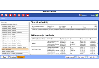
BrightStat output of the one-way ANOVA example
This is a fictitious example.
How to do this example on BrightStat webapp
Wiki link one-way ANOVA
Wiki link post hoc analysis
Wiki link Levene test for homogeneity of variances
References
Bortz, J. (2005). Statistik für Human- und Sozialwissenschaftler (6th Edition). Heidelberg: Springer Medizin Verlag.
Fisher, Ronald (1918). Studies in Crop Variation. I. An examination of the yield of dressed grain from Broadbalk. Journal of Agricultural Science, 11, 107–135. doi:10.1017/S0021859600003750
Scheffé, H. (1953). A method of judging all contrasts in the analysis of variance. Biometrika, 40, 87-104.
Tamhane, A.C. (1977). Multiple comparisons in model I one-way ANOVA with unequal variances. Communications in Statistics - Theory and Methods. 6(1), 15-32. doi:10.1080/03610927708827466
Levene, H. (1960). In:Contributions to Probability and Statistics: Essays in Honor of Harold Hotelling, I. Olkin et al. eds., Stanford University Press, 278-292.


 Donate IOTA